Calibration is the process of assigning a value, usually in concentration units, to an instrument response. For example, you might "calibrate" the response of a UV-visible absorption spectrometer (which is in units of absorbed light) by placing different "known" concentrations of analyte in a cell in the light path and establishing the instrument response per unit concentration. This "response function" should ideally be a straight line that passes directly through the origin. Why? Because it is unlikely that the unknown concentration, which you will determine by extrapolating the observed "unknown absorbance" over to the calibration function on the graph, will fall exactly on one of the known calibration points. Therefore you must know the calibration function exactly. A function of a line is exactly known, and physical phenomena that produce a linear response can be exactly modeled. On the other hand, if the calibration function was nonlinear, it would not be as easy to define and more sensitive to changes in physical phenomena. There would be greater error on any concentration determined from a nonlinear instrument response. So, what you want and what you most often see is a linear calibration function in analytical chemistry.

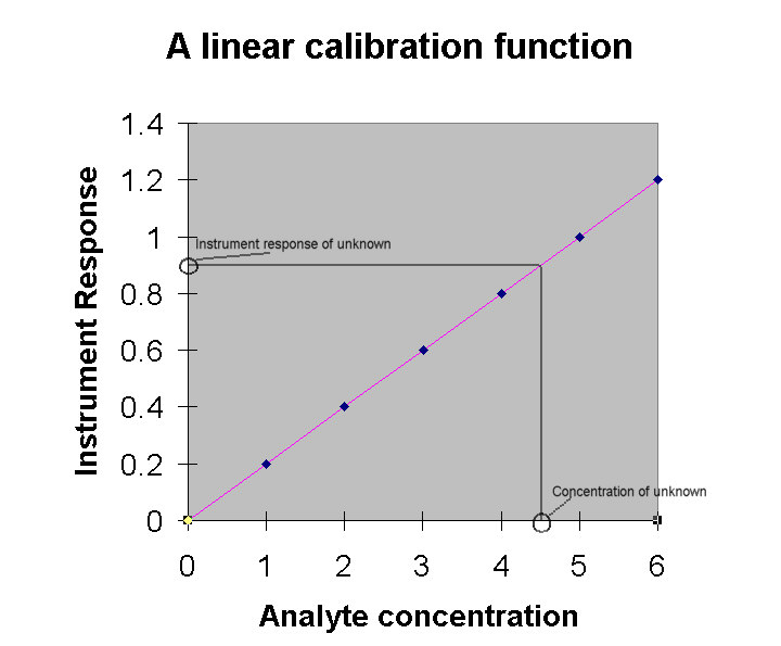
A line can be described by an equation: y = mx + b, where m is the slope of the line in terms of Dy/Dx (i.e., change in y/change in x). The intercept with the line of the y-axis is b. In terms of the graph shown above, we can convert y = mx + b to the terms:

The intercept is the "blank concentration" since it is the instrument response corresponding to an analyte concentration of zero. In the graph shown above, the calibration function is established based on 7 points as shown here:

Concentration	Instrument Response
0	0.000
1	0.200
2	0.400
3	0.600
4	0.800
5	1.000
6	1.200

The slope in this example would be 0.200 and the intercept would be 0. The equation of the line would therefore be:

Plug in a few values of x (instrument response) to the formula and you will see that it applies to the data set in the table on the previous page.

Normally, the points from which the calibration function is determined do not fit so well as shown in the previous table. In such a case, you use the linear regression function of a calculator or spreadsheet to give you a line of best fit. This calibration line will be defined by a slope and intercept, which will be given to you in the equation of the line. Let’s plot the following data set using the regression function of Excel (data analysis, regression):

Concentration	Instrument Response
0	0.025
1	0.217
2	0.388
3	0.634
4	0.777
5	1.011
6	1.166

You will note from the graph on the right that there is a considerable amount of scatter around the regression line, and that the intercept of the line on line on the y (instrument response) axis is not zero. This is the normal situation for analytical data and the result is that the use of a calibration line causes a certain amount of uncertainty in the concentrations determined from the calibration curve. This is discussed more fully in your textbook.

If, for example, we found that an unknown solution gave an instrument response of 0.254, we would enter that as y in the equation and solve for x:

What can go wrong with this "direct calibration" method? Two things: additive errors and multiplicative errors. An additive error is one that changes the intercept of the calibration function. Perhaps in the process of measuring the absorbance of a series of standards using a UV-vis absorption spectrophotometer, you unknowingly place a fingerprint on the absorption cell. Instead of a plot as shown above, you get a line that is offset from the origin on the y-axis by the instrument response resulting from the fingerprint. It will be the same at all analyte concentrations.

It is difficult to correct for an additive error if you don’t know that it exists. For example, in the calibration curve shown at the right, if the standards were measured in the cuvette with the fingerprint, but the cuvette was cleaned before the samples were measured, all the sample measurements would be in error by the instrument response due to the fingerprint. To the analyst, the calibration curve would look like the graph on the previous page (since the instrument zero is set with the standard blank), while it "really" looks like the graph on the right.

Careful experimental observations can sometimes detect additive errors. For example, in the aforementioned situation, if a sample blank were measured along with the samples, it would produce a negative instrument response, since there would be no fingerprint on the cuvette. That would be an immediate clue that there was an additive error in the standard measurements.

Another way to detect such an error is to repeat the calibration after all samples have been measured. Repetition is the key to good analytical results and the fact that the calibration line has shifted will become obvious when the standard measurements are repeated with a clean cell.

Additive errors can also result from the presence of a molecule (other than the analyte) in the sample that produces an instrument response (i.e., absorbs light) at the same wavelength as the molecule you are trying to determine. This extra absorption by the interfering molecule will make it appear that there is more of the molecule you are trying to measure than there actually is. This is a far more difficult problem to solve, although there are instrumental methods to deal with it.

Multiplicative interferences are those which change the slope of the calibration line. One example of a multiplicative interference might be if the cuvette used for the standards had a longer path length that that used for the samples. You may recall that in absorption spectrophotometry:

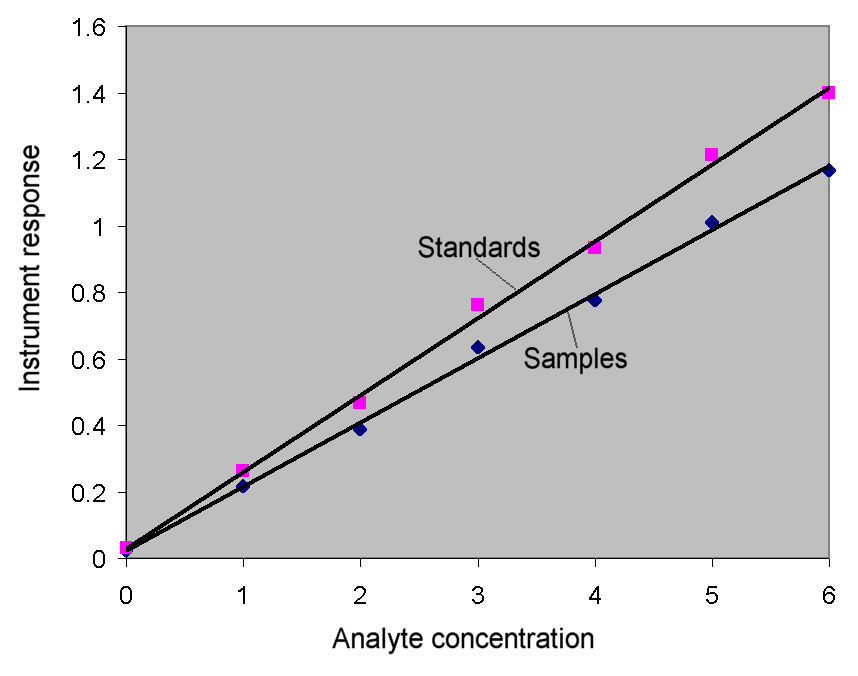Therefore, since the cuvette used for the standards has a longer path length, the sample absorbances will appear to represent concentrations that are lower than they actually are. The error on each sample measurement would constant on a relative basis (i.e., a 10% relative error … 10% too low.) This can be seen from the graph at the right. The curve with the greater slope is prepared using the standards (with the longer path length). Measurements of sample absorbance compared to this curve will give a concentration that is too low. The curve to which the samples should be compared has a lower slope. This curve would be generated from standards measured in the same cuvette as was used for the samples. The relative error between the two curves is approximately 10%.

The change in slope of the analytical curve caused by systematic errors such as using different cuvette path lengths can be referred to as a change in sensitivity … that is, a change in the instrument response per unit concentration. Such effects can be caused by other components of a sample matrix that enhance or depress the instrument response of the analyte in the sample matrix as compared to the instrument response of the analyte in the standards.

How do you correct for multiplicative errors? The best way is to use the method of standard addition, in which you add a known concentration of analyte to the unknown sample and then compare the increase of instrument response caused by the addition of the analyte to the instrument response observed for that concentration of analyte in the calibration standards.

The formula for the method of standard addition is:

where:

C_s = concentration of the sample (unknown)

C_a = concentration of the addition (known)

S_s = instrument response from the sample (known)

S_a = instrument response from the addition (known)

Solving for C_s will give the correct concentration for the analyte, corrected for multiplicative interferences. The method of standard addition also has the extra benefit that it will compensate for time drift of instrument response.

Another method of calibration that is useful in compensating for temporal (i.e., time) drift of instrument response as well as calibration curve nonlinearity is the method of bracketing. It is basically a simplified direct calibration where only 2 standards are used to establish the instrument response function. Bracketing is used when the instrument response varies with time. In such a case, a multi-point calibration line that was established at the beginning of an analysis would be invalid during the analysis because the slope of the calibration line changed while the samples were being measured. Essentially, two calibration points are chosen close to and on either side of the unknown sample signal and repeatedly measured. The calculation is as follows:

where:

C_U = concentration of unknown

C_L = concentration of low calibration standard

C_H = concentration of high calibration standard

S_U = instrument response from unknown

S_L = instrument response from C_L

S_H = instrument response from C_H

This may look complex, but all that is happening is that a slope is established between the low and high standards and the concentration of the unknown is determined based on the ratio of (S_U – S_L)/(S_H – S_L). Adding this concentration to the concentration of the low standard will give the concentration of the unknown sample.

To be continued with a discussion of internal standardization.